This website gives an overview of current communication standards utilizing Low Density Parity Check (LDPC) Forward Error Correction and an overview of the algorithms and architecture of LDPC encoder/decoder(s). In addition, an introduction to the design of LDPC codes and the issue of error floors and error floor mitigation is provided.
Standards utilizing LDPC
The following is a current list of standards that include LDPC FECs in their specification:
- DVB-X2 is the ETSI physical layer specification common to: terrestrial Digital Video Broadcasting (DVB-T2 2012), cable (DVB-C2 2016) and satellite (DVB-S2 2014). All 3 standards use the same LDPC codes.
- DVB-S2X is an optional extension to DVB-S2 with additional LDPC codes
- ETSI also has a GEO-Moble Radio (2008) interface specification that has LDPC FEC
- The DOCSIS 3.1 standard (2015) has added LDPC to its specification
- IEEE 802.11 (WiFi 2012) requires LDPC support in several of its sub-standards (e.g. 802.11ac, 802.11ad, 802.11ay)
- IEEE 1901 (2010) Broadband over powerline has optional LDPC
- IEEE 802.15.3c (2009) Wireless Personal Area Networks (WPAN) requires both RS and LDPC
- IEEE 802.3 (2012) 10 GBASE-T Ethernet specifies LDPC in section 55
- 16 (2012) WirelessMAN has LDPC as an option
- 22 (2011) Cognitive Wireless Regional Area Networks has a specification for LDPC
Introduction to FEC, ECC & LDPC
Forward Error Correction (FEC) is a technique used to protect data from errors by introducing redundant information through the use of Error Correcting Codes (ECC). Redundancy in the data representation provides two capabilities. The ability to detect that there are errors in the data and the possibility of correcting those errors. The data plus the redundant information is known as a codeword.
There are a variety of different families of FEC codes, each different algorithms. The two main categories of codes are block codes and convolutional codes. Block codes are fixed sized packets of data, and convolutional codes operate on streams of symbols. Block codes can be hard-decision or soft-decision. A hard-decision code is used for systems where only data bits are available, that is the bits have all been hard sliced into a 0 or a 1.
For soft-decision the slicer information is used to help the code make decisions. The closer the electrical signal is to the slice point the weaker the confidence that the slicer made the right decision. The farther from the slice point, the stronger the confidence the right decision was made. When decoding the codeword, the soft-decision decoder operates on both the data bit and its corresponding confidence values. This results in stronger code performance than basic hard-decision codes. The combined data bits and their confidence values are usually represented by Log-Likelihood Ratios (LLRs).
Low Density Parity Check (LDPC) codes are a popular class of capacity approaching, soft-decision block codes that was originally developed by Robert Gallager in 1963. Due to the computational complexity of the codes they remained largely unused until the late 1990s. With the advancement of VLSI and FPGA technologies and the rapid advancements in decoder architecture during the 2000s, LDPC has become the FEC of choice for high performance soft error correction.
- ITU-T G.9960 (2015) G.hn unified high-speed wireline home networking transceivers
Quasi-cyclic LDPC Codes
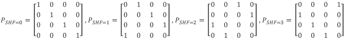
Each LDPC code is represented by an H-Matrix which specifies how the parity relates to the data. A common form of the H-matrix is called quasi-cyclic. In this form, the H-matrix is compressed into a matrix composed of sub-matrices. Each sub-matrix is a cyclically shifted identity matrix, represented by an integer value of the shift. The amount of data a single sub-matrix represents is known as the expansion factor (Z). Table 1 is an example of a quasi-cyclic H-matric from the 802.11ad WiGig standard with 4 rows and 16 cells per row. Each cell has an expansion factor of Z=42, e.g. each cell represents an identity submatrix cyclically shifted by the valued expressed in the cell.
If a submatrix is not part of the parity calculations for that row, it is represented by either a blank entry (as in the WiGig standard), or more commonly by a -1 or just a hyphen (-). Equation 1 demonstrates all the possible shifts of a sub-matrix with an expansion factor of Z=4. Note that a shift of zero is possible and means that the data represented by that cell is part of the parity calculations.
Table 1: WiGig rate 3/4 quasi-cyclic LDPC H-matrix:
| 35 | 19 | 41 | 22 | 40 | 41 | 39 | 6 | 28 | 18 | 17 | 3 | 28 | -1 | -1 | -1 |
| 29 | 30 | 0 | 8 | 33 | 22 | 17 | 4 | 27 | 28 | 20 | 27 | 24 | 23 | -1 | -1 |
| 37 | 31 | 18 | 23 | 11 | 21 | 6 | 20 | 32 | 9 | 12 | 29 | -1 | 0 | 13 | -1 |
| 25 | 22 | 4 | 34 | 31 | 3 | 14 | 15 | 4 | -1 | 14 | 18 | 13 | 13 | 22 | 24 |
Equation 1: Example of shifted sub - matrix with expansion factor of 4
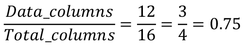
The rate of the code describes the amount of overhead that has been added to the data to produce a codeword. The code rate is specified as a fraction or a percent. The lower the code rate, the more overhead that is added to the code. Generally, the more overhead the better the code performs, i.e. the more errors it is capable of correcting. However, the lower the code rate, the less actual data that is transmitted per code word.
The codeword in Table 1 is 672 bits long, . The code has 12 data columns and 4 parity columns. Thus, the data size is 504 bits () and a parity size is 168 bits (). The code rate of the code is calculated as:
Equation 2: Calculating the code rate
LAYERED CODES
When discussing code matrices, a layer is a selection of orthogonal H-matrix rows that can be processed in parallel. As the rate of the code decrease the amount of parity needed increases. Orthogonal rows being packed into a layer is used to keep the code from gaining too many layers, and to provide a higher data to parity ratio. Each additional layer adds processing latency to every iteration within the decoder.
For example, the 4 row, ¾ rate WiGig code in Table 1 is run as a single row per layer (RPL). However, the 8 row, rate ½ rate code from the WiGig standard is a fully 2RPL code. Each of its eight rows are meant to be paired with another row so it runs in 4 layers. Thus an 8 row code and a 4 row code can process a full iteration of the algorithm in the same number of clock cycles. Mixed RPL codes are also possible, where some H-matrix rows are run on their own and others are run with a paired orthogonal row.
An orthogonal row is one that does not share any of the same columns of the H-matrix. Table 2 WiGig rate ½ code’s first and third rows. Note how none of the “on” columns overlap between the two rows. They can therefore be run in parallel together.
Table 2: First and third row of WiGig rate 1/2 code are orthogonal
| 40 | -1 | 38 | -1 | 13 | -1 | 5 | -1 | 18 | -1 | -1 | -1 | -1 | -1 | -1 | -1 |
| -1 | 36 | -1 | 31 | -1 | 7 | -1 | 34 | -1 | 10 | 41 | -1 | -1 | -1 | -1 | -1 |
LOG LIKELIHOOD RATIOS
Each bit in the decoder is represented by a Log Likelihood Ratio (LLR). This is a combination of the bit value and the confidence of that bit value. This quantity is represented in the sign/magnitude format, with the value of the bit being the sign and the magnitude the confidence. Thus a bit value of 1’b1 is a negative LLR and a bit value of 1’b0 is a positive LLR. The magnitude is a calculation based of the probability of the channel causing an error (Pe):
Example 3: Calculating Log Likelihood Ratio (LLR) Magnitudes
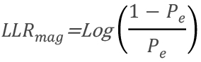
However, sometimes a static value is assigned to the zeroes and ones based on the expected operating error of the code rate.
DECODER STRUCTURE
Most of the effort in LDPC systems implementation is focused on the decoder. This is because of the significant asymmetry in the size between the decoder and encoder. The encoder is typically 10% of the area of a decoder for the same code family. However, the encoder can be made larger to increase the code performance with little or no increase to decoder area.
One of the more significant advancements in LDPC decoder architecture was the layered LDPC decoder. Despite the name, the layered decoder is unrelated to the layered codes mentioned earlier. The layered decoder can handle both layered and non-layered codes. The layered decoder has significantly better convergence than the traditional flood decoder.
The flood decoder is made up of 3 main processing blocks: the shifters, the variable nodes and the check nodes (see Figure 1). The codeword enters the shifters, which shift the data for processing according to values in the H-matrix. The data is then passed to the variable nodes, back to the shifter and then through the check nodes. This is a single iteration of a flood decoder. The check nodes compute the per layer parity checks for the code. The variable nodes are used to link the per layer bit decisions of the check nodes into a consolidated decision for the whole H-matrix. The check node also checks the parity equations within the codeword, which helps determine convergence. Once the check node parity equations fully pass the codeword has converged and is ready for release.
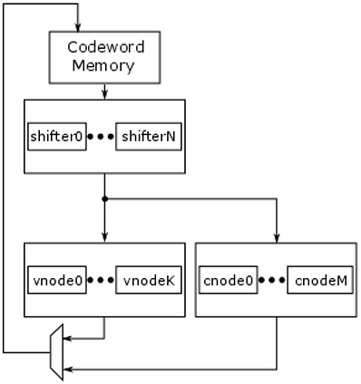
Figure 1: Basic flood decoder architecture
The layered decoder is made up of 2 main processing blocks: the shifters and the layered check node (see Figure 2). The layered check node structure includes the elements of the variable node found in the traditional architecture. The codeword enters the shifters, which behave as the flood decoder, and then passes through the layered check node. This single loop is a full iteration of the decoder. Codeword convergence and exit is handled similar to the flood decoder.
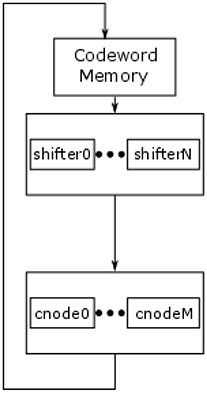
Figure 2: Basic layered decoder architecture
Most modern decoders are built using the layered decoder structure. This structure offers two main benefits. First, it is easier to schedule for full processing core utilization. Second, and more importantly, it has faster convergence. This means lower latency, higher throughput and lower power for every codeword processed.
LDPC Codes
The design of high quality LDPC is a non-trivial N-P complete problem. Poor code design results in error floors, higher power and latency and lower throughput. The design of LDPC codes tends to focus maximizing the girth of the code. The girth of a code is the length of the smallest cycle with in the Tanner graph of the code.
A problem with many code design algorithms is that they do not take into account the LDPC encoder and LDPC decoder hardware cost of the designed codes
There are a number of algorithms that have been developed to assist in the design of quality LDPC codes:
* Progressive Edge Growth (PEG) – an algorithm that operates on the Tanner graph to produce codes with large girth
* Approximate Cycle EMD (ACE) – another Tanner graph algorithm that focuses on multiple cycles. Can be combined with PEG to get a hybrid result.
* Accumulator Based Codes – An approach that tries to produce efficiently encodeable codes. Can also be used for turbo codes. Used to produce 2 of the codes used in the DVB S2 standard.
* Finite Geometry (FG) LDPC – a class of code construction techniques used to generate LDPC codes algebraically.
* Finite Field Construction – Another class of code construction algorithms. The Structured RS-LDPC technique was used to produce the 10Gbit Ethernet standard codes based on Reed-Solomon codes.
Error Floors
There are a number of factors that can cause error floors. An error floor occurs when a reduction in noise (errors) in does not result in an improved coding performance. It can also be a less than expected improvement due to a reduction in noise (i.e. an inflection point in the performance curve).
Possible causes of error floors are:
* Trapping sets – a trapping set is a pattern of variable and check nodes within the code that when in error cause the code word to decode into a near code word.
* Quantized Arithmetic Floors – even in well-designed systems quantization effects can cause decode problems at very low error rates.
Careful code design can reduce error floors and significant decoder performance can be gained relative to commercially available standard based codes such as WiGig, WiMax or WiFi. Custom code design is also required for applications such as Flash storage which require extremely stringent error floor performance
Eideticom
The team at Eideticom has over 15 years of experience designing high performance ECC / FEC systems, with almost a decade focused on LDPC systems and code design.